Homework 12 - The Runge-Kutta ODE Solver

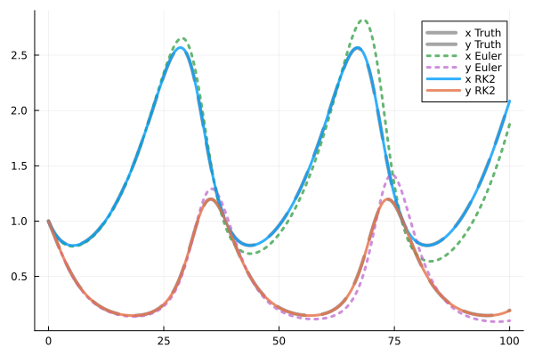
There exist many different ODE solvers. To demonstrate how we can get significantly better results with a simple update to Euler, you will implement the second order Runge-Kutta method RK2:

\begin{aligned} {\tilde{x}}_{n + 1} & = x_{n} + h f (x_{n}, t_{n}) \\ x_{n + 1} & = x_{n} + \frac{h}{2} (f (x_{n}, t_{n}) + f ({\tilde{x}}_{n + 1}, t_{n + 1})) \end{aligned}

RK2 is a 2nd order method. It uses not only $f$ (the slope at a given point), but also $f^{'}$ (the derivative of the slope). With some clever manipulations you can arrive at the equations above with make use of $f^{'}$ without needing an explicit expression for it (if you want to know how, see here). Essentially, RK2 computes an initial guess 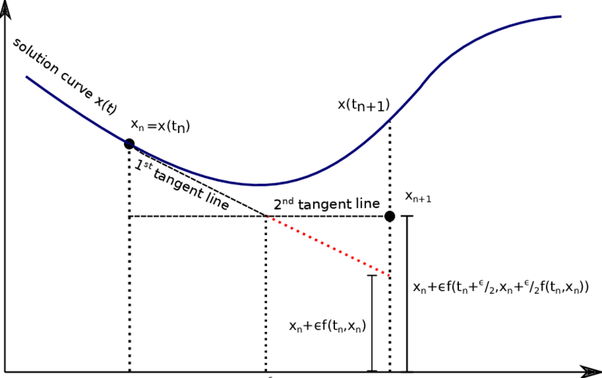${\tilde{x}}_{n + 1}$ to then average the slopes at the current point $x_{n}$ and at the guess ${\tilde{x}}_{n + 1}$ which is illustarted below.

The code from the lab that you will need for this homework is given below. As always, put all your code in a file called hw.jl, zip it, and upload it to BRUTE.

julia

struct ODEProblem{F,T<:Tuple{Number,Number},U<:AbstractVector,P<:AbstractVector}
    f::F
    tspan::T
    u0::U
    θ::P
end


abstract type ODESolver end

struct Euler{T} <: ODESolver
    dt::T
end

function (solver::Euler)(prob::ODEProblem, u, t)
    f, θ, dt  = prob.f, prob.θ, solver.dt
    (u + dt*f(u,θ), t+dt)
end


function solve(prob::ODEProblem, solver::ODESolver)
    t = prob.tspan[1]; u = prob.u0
    us = [u]; ts = [t]
    while t < prob.tspan[2]
        (u,t) = solver(prob, u, t)
        push!(us,u)
        push!(ts,t)
    end
    ts, reduce(hcat,us)
end


# Define & Solve ODE

function lotkavolterra(x,θ)
    α, β, γ, δ = θ
    x₁, x₂ = x

    dx₁ = α*x₁ - β*x₁*x₂
    dx₂ = δ*x₁*x₂ - γ*x₂

    [dx₁, dx₂]
end

lotkavolterra (generic function with 1 method)

Homework (2 points)

Implement the 2nd order Runge-Kutta solver according to the equations given above by overloading the call method of a new type RK2.

julia

(solver::RK2)(prob::ODEProblem, u, t)

You should be able to use it exactly like our Euler solver before:

julia

using Plots
using JLD2

# Define ODE
function lotkavolterra(x,θ)
    α, β, γ, δ = θ
    x₁, x₂ = x

    dx₁ = α*x₁ - β*x₁*x₂
    dx₂ = δ*x₁*x₂ - γ*x₂

    [dx₁, dx₂]
end

θ = [0.1,0.2,0.3,0.2]
u0 = [1.0,1.0]
tspan = (0.,100.)
prob = ODEProblem(lotkavolterra,tspan,u0,θ)

# load correct data
true_data = load("lotkadata.jld2")

# create plot
p1 = plot(true_data["t"], true_data["u"][1,:], lw=4, ls=:dash, alpha=0.7,
          color=:gray, label="x Truth")
plot!(p1, true_data["t"], true_data["u"][2,:], lw=4, ls=:dash, alpha=0.7,
      color=:gray, label="y Truth")

# Euler solve
(t,X) = solve(prob, Euler(0.2))
plot!(p1,t,X[1,:], color=3, lw=3, alpha=0.8, label="x Euler", ls=:dot)
plot!(p1,t,X[2,:], color=4, lw=3, alpha=0.8, label="y Euler", ls=:dot)

# RK2 solve
(t,X) = solve(prob, RK2(0.2))
plot!(p1,t,X[1,:], color=1, lw=3, alpha=0.8, label="x RK2")
plot!(p1,t,X[2,:], color=2, lw=3, alpha=0.8, label="y RK2")

Homework 12 - The Runge-Kutta ODE Solver ​

Homework 12 - The Runge-Kutta ODE Solver