Lab 11: GPU programming

In this lab we are going to delve into GPU acceleration. Julia offers a unified interface to the four most important GPU vendors via four separate packages:

• CUDA.jl
• AMDGPU.jl
• oneAPI.jl (Intel's oneAPI toolkit)
• Metal.jl (targets Apple's M-series chips)

Array programming

We can do quite a lot without even knowing that we are using GPU instead of CPU. This marvel is the combination of Julia's multiple dispatch and array abstractions. In many cases it will be enough to move your CPU array to the appropriate GPU array:

using MyGPUPackage

a = rand(Float32, 1024) |> MyGPUArray

sin.(a) |> sum

Based on the size of the problem and intricacy of the computation we may be achieve both incredible speedups as well as slowdowns.

All four above mentioned pacakages have (almost) the same interfaces, which offer the following user facing functionalities

• device management versioninfo, device!
• definition of arrays on gpu (e.g. CuArray or MtlArray)
• data copying from host(CPU) to device(GPU) and the other way around
• wrapping already existing library code in CuBLAS, CuRAND, CuDNN, CuSparse and others
• kernel based programming (more on this in the second half of the lab)

Let's use this to inspect our GPU hardware.

julia> using Metal

julia> Metal.versioninfo()
macOS 14.2.1, Darwin 23.2.0

Toolchain:
- Julia: 1.9.4
- LLVM: 14.0.6

Julia packages: 
- Metal.jl: 0.5.1
- Metal_LLVM_Tools_jll: 0.5.1+0

1 device:
- Apple M1 Pro (2.608 GiB allocated)

As we have already seen in the lecture, we can simply import e.g. Metal.jl define some arrays, move them to the GPU and do some computation. In the following code we define two matrices 1000x1000 filled with random numbers and multiply them using usual x * y syntax.

using Metal

x = randn(Float32, 60, 60)
y = randn(Float32, 60, 60)

mx = MtlArray(x)
my = MtlArray(y)

@info "" x*y ≈ Matrix(mx*my)

┌ Info:
└   x * y ≈ Matrix(mx * my) = true

This may not be anything remarkable, as such functionality is available in many other languages albeit usually with a less mathematical notation like x.dot(y). With Julia's multiple dispatch, we can simply dispatch the multiplication operator/function * to a specific method that works on MtlArray type. You can check with @code_typed:

julia> @code_typed mx * my
CodeInfo(
1 ─ %1 = Base.getfield(A, :dims)::Tuple{Int64, Int64}
│   %2 = Base.getfield(%1, 1, true)::Int64
│   %3 = Base.getfield(B, :dims)::Tuple{Int64, Int64}
│   %4 = Base.getfield(%3, 2, true)::Int64
│   %5 = Core.tuple(%2, %4)::Tuple{Int64, Int64}
│   %6 = LinearAlgebra.similar::typeof(similar)
│   %7 = invoke Metal.:(var"#similar#30")($(QuoteNode(Metal.MTL.MTLResourceStorageModePrivate))::Metal.MTL.MTLResourceOptions, %6::typeof(similar), B::Metal.MtlMatrix{Float32, Metal.MTL.MTLResourceStorageModePrivate}, Float32::Type{Float32}, %5::Tuple{Int64, Int64})::Metal.MtlMatrix{Float32}
│   %8 = LinearAlgebra.gemm_wrapper!(%7, 'N', 'N', A, B, $(QuoteNode(LinearAlgebra.MulAddMul{true, true, Bool, Bool}(true, false))))::Metal.MtlMatrix{Float32}
└──      return %8
) => Metal.MtlMatrix{Float32}

Let's now explore what the we can do with this array programming paradigm on some practical examples.

# using Pkg; 
# Pkg.add(["FileIO", "ImageMagick", "ImageShow", "ColorTypes"])

# using FileIO, ImageMagick, ImageShow, ColorTypes
#
# rgb_img = FileIO.load("image.jpeg");
# gray_img = Float32.(Gray.(rgb_img));
gray_img = rand(Float32, 10000, 10000)
cgray_img = MtlArray(gray_img)

julia> cimg
┌ Warning: Performing scalar indexing on task Task (runnable) @0x00007f25931b6380.
│ Invocation of getindex resulted in scalar indexing of a GPU array.
│ This is typically caused by calling an iterating implementation of a method.
│ Such implementations *do not* execute on the GPU, but very slowly on the CPU,
│ and therefore are only permitted from the REPL for prototyping purposes.
│ If you did intend to index this array, annotate the caller with @allowscalar.
└ @ GPUArrays ~/.julia/packages/GPUArrays/gkF6S/src/host/indexing.jl:56
julia> Array(cimg)
Voila!
julia> cimg;

negative(i) = 1.0f0 .- i
darken(i) = i .* 0.5f0
brightest(i) = findmax(i)

julia> using BenchmarkTools

julia> @btime Metal.@sync negative($cgray_img);
  53.253 ms (295 allocations: 7.68 KiB)

julia> @btime negative($gray_img);
  37.857 ms (2 allocations: 381.47 MiB)

julia> @btime Metal.@sync darken($cgray_img);
  52.056 ms (311 allocations: 7.99 KiB)

julia> @btime darken($gray_img);
  39.182 ms (2 allocations: 381.47 MiB)

julia> @btime Metal.@sync brightest($cgray_img);
  43.543 ms (1359 allocations: 34.91 KiB)

julia> @btime brightest($gray_img);
  124.636 ms (0 allocations: 0 bytes)

In the next example we will try to solve a system of linear equations $Ax=b$, where A is a large (possibly sparse) matrix.

α = 10.0f0
β = 10.0f0

function init(N, α, β, r = (0.f0, π/2.0f0))
    dx = (r[2] - r[1]) / N
    A = zeros(Float32, N+2, N+2)
    A[1,1] = 1.0f0
    A[end,end] = 1.0f0
    for i in 2:N+1
        A[i,i-1] = 1.0f0/(dx*dx)
        A[i,i] = -2.0f0/(dx*dx) - 16.0f0
        A[i,i+1] = 1.0f0/(dx*dx)
    end

    b = fill(-8.0f0, N+2)
    b[1] = α
    b[end] = β
    A, b
end

N = 30
A, b = init(N, α, β)

A, b = init(N, α, β)
cA, cb = CuArray(A), CuArray(b)
A
b
A\b
cA\cb

@btime $A \ $b;
@btime CUDA.@sync Array(CuArray($A) \ CuArray($b));

Programming GPUs in this way is akin to using NumPy, MATLAB and other array based toolkits, which force users not to use for loops. There are attempts to make GPU programming in Julia more powerful without delving deeper into writing of GPU kernels. One of the attempts is Tulio.jl, which uses macros to annotate parallel for loops, similar to OpenMP's pragma intrinsics, which can be compiled to GPU as well.

Note also that Julia's CUDA.jl is not a tensor compiler. With the exception of broadcast fusion, which is easily transferable to GPUs, there is no optimization between different kernels from the compiler point of view. Furthermore, memory allocations on GPU are handled by Julia's GC, which is single threaded and often not as aggressive, therefore similar application code can have different memory footprints on the GPU.

Nowadays there is a big push towards simplifying programming of GPUs, mainly in the machine learning community, which often requires switching between running on GPU/CPU to be a one click deal. However this may not always yield the required results, because the GPU's computation model is different from the CPU, see lecture. This being said e.g. Julia's Flux.jl framework does offer such capabilities ^[2]

using Flux, CUDA
m = Dense(10,5) |> gpu
x = rand(10) |> gpu
y = m(x)
y |> cpu

Kernel programming

There are two paths that lead to the necessity of programming GPUs more directly via kernels

1. We cannot express our algorithm in terms of array operations.
2. We want to get more out of the code,

Note that the ability to write kernels in the language of your choice is not granted, as this club includes a limited amount of members - C, C++, Fortran, Julia ^[3]. Consider then the following comparison between CUDA C and CUDA.jl implementation of a simple vector addition kernels as seen in the lecture.

#define cudaCall(err) // check return code for error
#define frand() (float)rand() / (float)(RAND_MAX)

__global__ void vadd(const float *a, const float *b, float *c) {
	int i = blockIdx.x * blockDim.x + threadIdx.x;
	c[i] = a[i] + b[i];
}

const int len = 100;
int main() {
	float *a, *b;
	a = new float[len];
	b = new float[len];
	for (int i = 0; i < len; i++) {
		a[i] = frand(); b[i] = frand();
	}
	float *d_a, *d_b, *d_c;
	cudaCall(cudaMalloc(&d_a, len * sizeof(float)));
	cudaCall(cudaMemcpy(d_a, a, len * sizeof(float), cudaMemcpyHostToDevice));
	cudaCall(cudaMalloc(&d_b, len * sizeof(float)));

	cudaCall(cudaMemcpy(d_b, b, len * sizeof(float), cudaMemcpyHostToDevice));
	cudaCall(cudaMalloc(&d_c, len * sizeof(float)));

	vadd<<<1, len>>>(d_a, d_b, d_c);

	float *c = new float[len];
	cudaCall(cudaMemcpy(c, d_c, len * sizeof(float), cudaMemcpyDeviceToHost));
	cudaCall(cudaFree(d_c));
	cudaCall(cudaFree(d_b));
	cudaCall(cudaFree(d_a));

	return 0;
}

Compared to CUDA C the code is less bloated, while having the same functionality.^[4]

function vadd(a, b, c)
    # CUDA.jl
    # i = (blockIdx().x-1) * blockDim().x + threadIdx().x

    # Metal.jl
    i = thread_position_in_grid_1d()
	c[i] = a[i] + b[i]

	return
end

len = 100
a = rand(Float32, len)
b = rand(Float32, len)
d_a = MtlArray(a)
d_b = MtlArray(b)
d_c = similar(d_a)
@metal threads = len vadd(d_a, d_b, d_c)
c = Array(d_c)

You can check what instructions are implemented by your custom kernel via GPU specific introspection macros:

julia> @device_code_agx @metal threads = len vadd(d_a, d_b, d_c)
; GPUCompiler.CompilerJob{GPUCompiler.MetalCompilerTarget, Metal.MetalCompilerParams}(MethodInstance for vadd(::MtlDeviceVector{Float32, 1}, ::MtlDeviceVector{Float32, 1}, ::MtlDeviceVector{Float32, 1}), CompilerConfig for GPUCompiler.MetalCompilerTarget, 0x00000000000082f7)

___Z4vadd14MtlDeviceArrayI7Float32Li1ELi1EES_IS0_Li1ELi1EES_IS0_Li1ELi1EE._agc.main:
   0: 0511100d00c43200     device_load      0, i32, xy, r2_r3, u0_u1, 1, signed, lsl 1
   8: 3800                 wait             0
   a: f2151004             get_sr           r5.cache, sr80 (thread_position_in_grid.x)
   e: 9204840200010150     icmpsel          ugt, r1l.cache, r2.cache, 0, 1, 0
  16: 92028602000101d0     icmpsel          sgt, r0h.cache, r3.cache, 0, 1, 0
  1e: 9202860200c2108c     icmpsel          seq, r0h.cache, r3.cache, 0, r1l.discard, r0h.discard
  26: 8e0501a028000000     iadd             r1.cache, 1, r5.cache
  2e: 921981000000418c     icmpsel          seq, r6.cache, r0h.cache, 0, 0, r2.discard
  36: 9209c1000000618c     icmpsel          seq, r2.cache, r0h.discard, 0, 0, r3.discard
  3e: 920ccc2228010130     icmpsel          ult, r3l.cache, r6.discard, r1.cache, 1, 0
  46: 9202840200010130     icmpsel          ult, r0h.cache, r2.cache, 0, 1, 0
  4e: 9202c40200c6108c     icmpsel          seq, r0h.cache, r2.discard, 0, r3l.discard, r0h.discard
  56: 920842a22c010130     icmpsel          ult, r2l.cache, r1, r5.discard, 1, 0
  5e: 9202c10000c41090     icmpsel          seq, r0h.cache, r0h.discard, 0, r2l.discard, 1
  66: e2000000             mov_imm          r0l.cache, 0
  6a: 5288c1000000         if_icmp          r0l, seq, r0h.discard, 0, 1
  70: 20c0b6000000         jmp_exec_none    0x126
  76: 0511140d00c43200     device_load      0, i32, xy, r2_r3, u2_u3, 1, signed, lsl 1
  7e: 3800                 wait             0
  80: 9210840200010150     icmpsel          ugt, r4l.cache, r2.cache, 0, 1, 0
  88: 92028602000101d0     icmpsel          sgt, r0h.cache, r3.cache, 0, 1, 0
  90: 9202860200c8108c     icmpsel          seq, r0h.cache, r3.cache, 0, r4l.discard, r0h.discard
  98: 921581000000418c     icmpsel          seq, r5.cache, r0h.cache, 0, 0, r2.discard
  a0: 9209c1000000618c     icmpsel          seq, r2.cache, r0h.discard, 0, 0, r3.discard
  a8: 920cca2224010130     icmpsel          ult, r3l.cache, r5.discard, r1, 1, 0
  b0: 9202840200010130     icmpsel          ult, r0h.cache, r2.cache, 0, 1, 0
  b8: 9202c40200c6108c     icmpsel          seq, r0h.cache, r2.discard, 0, r3l.discard, r0h.discard
  c0: 9202c10000001190     icmpsel          seq, r0h.cache, r0h.discard, 0, 0, 1
  c8: 5288c1000000         if_icmp          r0l, seq, r0h.discard, 0, 1
  ce: 20c058000000         jmp_exec_none    0x126
  d4: 0511180d00c43200     device_load      0, i32, xy, r2_r3, u4_u5, 1, signed, lsl 1
  dc: 3800                 wait             0
  de: 9210840200010150     icmpsel          ugt, r4l.cache, r2.cache, 0, 1, 0
  e6: 92028602000101d0     icmpsel          sgt, r0h.cache, r3.cache, 0, 1, 0
  ee: 9202860200c8108c     icmpsel          seq, r0h.cache, r3.cache, 0, r4l.discard, r0h.discard
  f6: 921581000000418c     icmpsel          seq, r5.cache, r0h.cache, 0, 0, r2.discard
  fe: 9209c1000000618c     icmpsel          seq, r2.cache, r0h.discard, 0, 0, r3.discard
 106: 9204ca222c010130     icmpsel          ult, r1l.cache, r5.discard, r1.discard, 1, 0
 10e: 9202840200010130     icmpsel          ult, r0h.cache, r2.cache, 0, 1, 0
 116: 9202c40200c2108c     icmpsel          seq, r0h.cache, r2.discard, 0, r1l.discard, r0h.discard
 11e: 1202c10000001190     icmpsel          seq, r0h, r0h.discard, 0, 0, 1
 126: 521600000000         pop_exec         r0l, 2
 12c: 721d1004             get_sr           r7, sr80 (thread_position_in_grid.x)
 130: 0529000d00c43200     device_load      0, i32, xy, r5_r6, u0_u1, 0, signed, lsl 1
 138: 0509040d00c43200     device_load      0, i32, xy, r1_r2, u2_u3, 0, signed, lsl 1
 140: 3800                 wait             0
 142: 0519ea0400c01200     device_load      0, i32, x, r3, r5_r6, r7, signed
 14a: 0529e20400c01200     device_load      0, i32, x, r5, r1_r2, r7, signed
 152: 0509080d00c43200     device_load      0, i32, xy, r1_r2, u4_u5, 0, signed, lsl 1
 15a: 3800                 wait             0
 15c: 2a8dc6a22c00         fadd32           r3, r3.discard, r5.discard
 162: 4519e20400c01200     device_store     0, i32, x, r3, r1_r2, r7, signed, 0
 16a: 8800                 stop

CUDA programming model

Recalling from the lecture, in CUDA's programming model, you usually write kernels, which represent the body of some parallel for loop.

• A kernel is executed on multiple threads, which are grouped into thread blocks.
• All threads in a block are executed in the same Streaming Multi-processor (SM), having access to some shared pool of memory.
• The number of threads launched is always a multiple of 32 (32 threads = 1 warp, therefore length of a thread block should be divisible by 32).
• All threads in a single warp are executed simultaneously.
• We have to take care of how many threads will be launched in order to complete the task at hand, i.e. if there are insufficiently many threads/blocks spawned we may end up doing only part of the task.
• We can spawn threads/thread blocks in both in 1D, 2D or 3D blocks, which may ease the indexing inside the kernel when dealing with higher dimensional data.

Thread indexing

Stopping for a moment here to illustrate the last point with a visual aid^[5]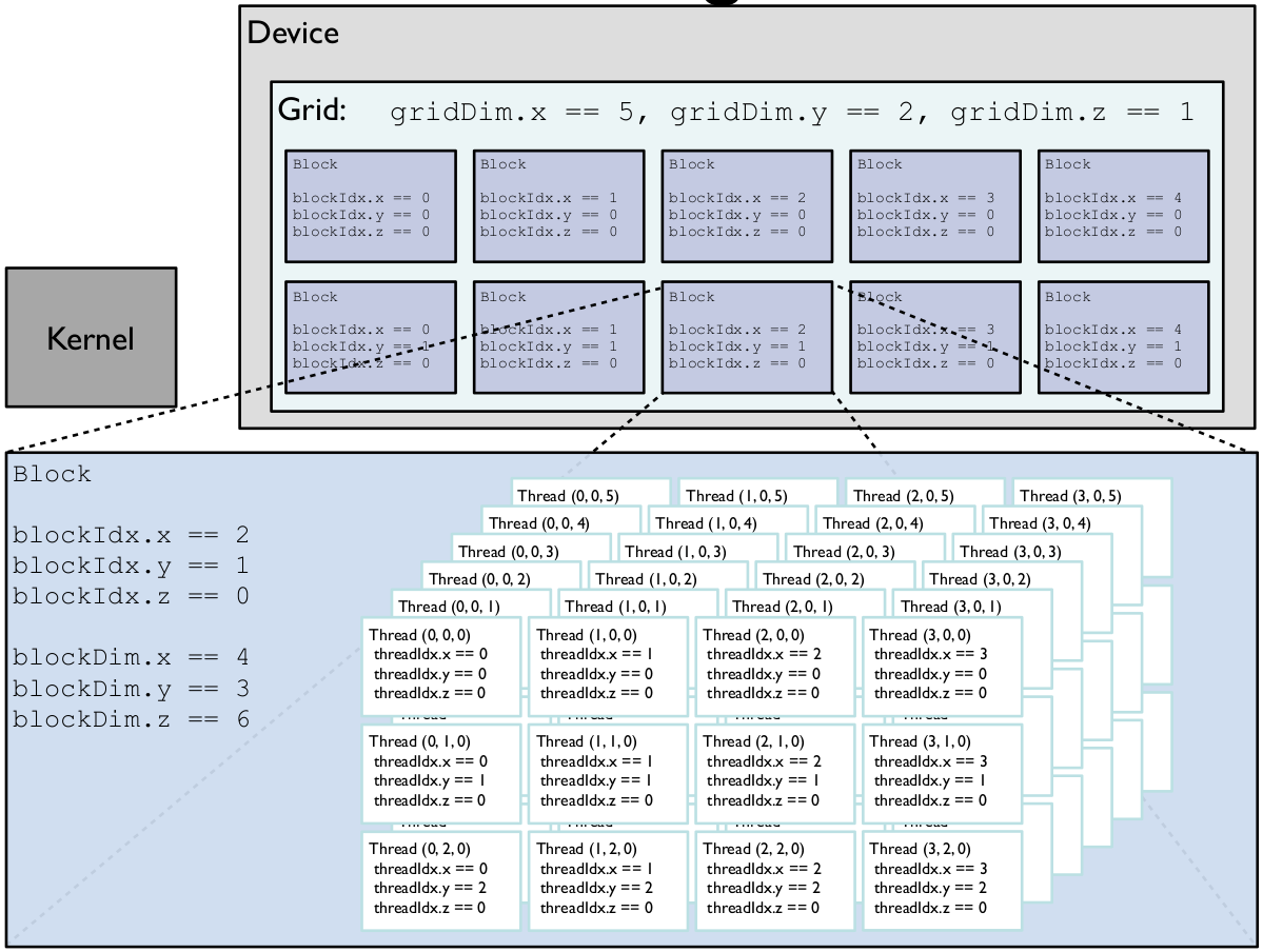

This explains the indexing into a linear array from above

i = (blockIdx().x-1) * blockDim().x + threadIdx().x

which is similar to the computation a linear index of multidimensional (in our case 2D array row ~ blockIdx and column threadIdx). Again let's use a visual help for this 1D vector^[6]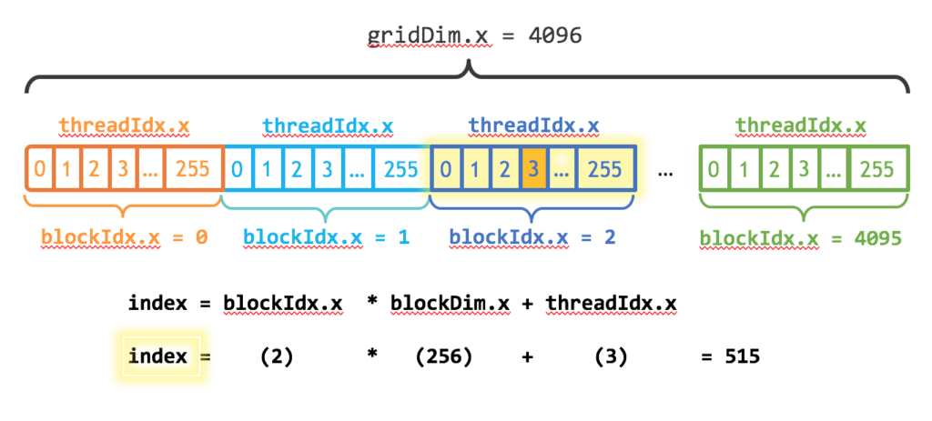

Launching a kernel

Let's now dig into what is happening during execution of the line @cuda threads = (1, len) vadd(d_a, d_b, d_c):

1. Compile the vadd kernel to GPU code (via LLVM and it's NVPTX backend)
2. Parse and construct launch configuration of the kernel. Here we are creating 1 thread block with 1x100 threads (in reality 128 threads may be launched).
3. Schedule to run vadd kernel with constructed launch configuration and arguments.
4. Return the task status.

It's important to stress that we only schedule the kernel to run, however in order to get the result we have to first wait for the completion. This can be done either via

• CUDA.@sync, which we have already seen earlier
• or a command to copy result to host (Array(c)), which always synchronizes kernels beforehand

@cuda threads=64 blocks=2 vadd(d_a, d_b, d_c)
@cuda threads=32 blocks=4 vadd(d_a, d_b, d_c)

@cuda threads=32 blocks=2 vadd(d_a, d_b, d_c)

function do_something(a,b)
	function do_something_kernel!(c,a,b)
		...
	end

	# handle allocation
	# handle launch configuration
	@cuda ... do_something_kernel!(c,a,b)
end

k = @cuda vadd(d_a, d_b, d_c)
CUDA.maxthreads(k)

function vadd(a, b, c)
	i = (blockIdx().x-1) * blockDim().x + threadIdx().x
    if i <= length(c)
	    c[i] = a[i] + b[i]
    end
	return
end

d_c = similar(d_a)
@cuda threads=32 blocks=2 vadd(d_a, d_b, d_c) # insufficient number of threads
Array(d_c)

len = 10_000
a = rand(Float32, len)
b = rand(Float32, len)
d_a = CuArray(a)
d_b = CuArray(b)
d_c = similar(d_a)

julia> @btime CUDA.@sync @cuda threads=256 blocks=cld(len, 256) vadd($d_a, $d_b, $d_c)
       @btime CUDA.@sync @cuda threads=128 blocks=cld(len, 128) vadd($d_a, $d_b, $d_c)
       @btime CUDA.@sync @cuda threads=64 blocks=cld(len, 64) vadd($d_a, $d_b, $d_c)
       @btime CUDA.@sync @cuda threads=32 blocks=cld(len, 32) vadd($d_a, $d_b, $d_c)
  8.447 μs (24 allocations: 1.22 KiB)
  8.433 μs (24 allocations: 1.22 KiB)
  8.550 μs (24 allocations: 1.22 KiB)
  8.634 μs (24 allocations: 1.22 KiB)

The launch configuration depends heavily on user's hardware and the actual computation in the kernel, where in some cases having more threads in a block is better (up to some point).

Image processing with kernels

Following up on exercise with image processing let's use kernels for some functions that cannot be easily expressed as array operations.

using CUDA
function translate_kernel!(output, input, translation)
    x_idx = (blockIdx().x-1) * blockDim().x + threadIdx().x
    y_idx = (blockIdx().y-1) * blockDim().y + threadIdx().y

    x_outidx = x_idx + translation[1]
    y_outidx = y_idx + translation[2]

    if (1 <= x_outidx <= size(output,1)) && 
        (1 <= y_outidx <= size(output,2)) && 
        (x_idx <= size(output,1)) && (y_idx <= size(output,2))
        output[x_outidx, y_outidx] = input[x_idx, y_idx]
    end

    return
end

using FileIO, ImageMagick, ImageShow, ColorTypes
rgb_img = FileIO.load("tape.jpeg");
gray_img = Float32.(Gray.(rgb_img));
cgray_img = CuArray(gray_img);
cgray_img_moved = CUDA.fill(0.0f0, size(cgray_img));

blocks = cld.((size(cgray_img,1), size(cgray_img,2)), 32)
@cuda threads=(32, 32) blocks=blocks translate_kernel!(cgray_img_moved, cgray_img, (100, -100))
Gray.(Array(cgray_img_moved))

#@cuda threads=(64, 64) blocks=(1,1) translate_kernel!(cgray_img_moved, cgray_img, (-500, 500)) # too many threads per block (fails on some weird exception) - CUDA error: invalid argument (code 1, ERROR_INVALID_VALUE)

Profiling

CUDA framework offers a wide variety of developer tooling for debugging and profiling our own kernels. In this section we will focus profiling using the Nsight Systems software that you can download after registering here. It contains both nsys profiler as well as nsys-uiGUI application for viewing the results. First we have to run julia using nsys application.

• on Windows with PowerShell (available on the lab computers)

& "C:\Program Files\NVIDIA Corporation\Nsight Systems 2021.2.4\target-windows-x64\nsys.exe" launch --trace=cuda,nvtx H:/Downloads/julia-1.6.3/bin/julia.exe --color=yes --color=yes --project=$((Get-Item .).FullName)

• on Linux

/full/path/to/nsys launch --trace=cuda,nvtx /home/honza/Apps/julia-1.6.5/bin/julia --color=yes --project=.

Once julia starts we have to additionally (on the lab computers, where we cannot modify env path) instruct CUDA.jl, where nsys.exe is located.

ENV["JULIA_CUDA_NSYS"] = "C:\\Program Files\\NVIDIA Corporation\\Nsight Systems 2021.2.4\\target-windows-x64\\nsys.exe"

Now we should be ready to start profiling our kernels.

CUDA.@profile CUDA.@sync begin 
    NVTX.@range "something" begin
    		# run some kernel
    end 

    NVTX.@range "something" begin
    		# run some kernel
    end 
end

CUDA.@profile CUDA.@sync begin
    NVTX.@range "copy H2D" begin
        rgb_img = FileIO.load("image.jpg");
        gray_img = Float32.(Gray.(rgb_img));
        cgray_img = CuArray(gray_img);
    end

    NVTX.@range "negative" begin 
        negative(cgray_img);
    end
    NVTX.@range "darken" begin 
        darken(cgray_img);
    end
    NVTX.@range "fourier" begin 
        fourier(cgray_img);
    end
    NVTX.@range "brightest" begin 
        brightest(cgray_img);
    end
end

Matrix multiplication

max_threads = 256
threads_x = min(max_threads, size(C,1))
threads_y = min(max_threads ÷ threads_x, size(C,2))
threads = (threads_x, threads_y)
blocks = ceil.(Int, (size(C,1), size(C,2)) ./ threads)

function generic_matmatmul!(C, A, B)
    function kernel(C, A, B)
        i = (blockIdx().x-1) * blockDim().x + threadIdx().x
        j = (blockIdx().y-1) * blockDim().y + threadIdx().y

        if i <= size(A,1) && j <= size(B,2)
            Ctmp = 0.0f0
            for k in 1:size(A,2)
                Ctmp += A[i, k]*B[k, j]
            end
            C[i,j] = Ctmp
        end

        return
    end

    max_threads = 256
    threads_x = min(max_threads, size(C,1))
    threads_y = min(max_threads ÷ threads_x, size(C,2))
    threads = (threads_x, threads_y)
    blocks = ceil.(Int, (size(C,1), size(C,2)) ./ threads)

    @cuda threads=threads blocks=blocks kernel(C, A, B)

    C
end

K, L, M = 10 .* (200, 100, 50)
A = CuArray(randn(K, L));
B = CuArray(randn(L, M));
C = similar(A, K, M);

generic_matmatmul!(C, A, B)

using LinearAlgebra
CC = similar(A, K, M)
mul!(CC, A, B)


using BenchmarkTools
@btime CUDA.@sync generic_matmatmul!(C, A, B);
@btime CUDA.@sync mul!(CC, A, B);

GPU vendor agnostic code

There is an interesting direction that is allowed with the high level abstraction of Julia - KernelAbstractions.jl, which offer an overarching API over CUDA, AMD ROCM and Intel oneAPI frameworks.

using KernelAbstractions

# Simple kernel for matrix multiplication
@kernel function matmul_kernel!(a, b, c)
    i, j = @index(Global, NTuple)

    # creating a temporary sum variable for matrix multiplication
    tmp_sum = zero(eltype(c))
    for k = 1:size(a)[2]
        tmp_sum += a[i,k] * b[k, j]
    end

    c[i,j] = tmp_sum
end

# Create a wrapper kernel which selects the correct backend
function matmul!(a, b, c)
    backend = KernelAbstractions.get_backend(a)
    kernel! = matmul_kernel!(backend)
    kernel!(a, b, c, ndrange=size(c))
end

using Metal
a = rand(Float32, 1000, 1000)
b = rand(Float32, 1000, 1000)
ag = a |> MtlArray
bg = b |> MtlArray
c = similar(ag)
matmul!(ag,bg,c)

@assert a*b ≈ Matrix(c)